Page 451 - Computer Software Application TP - Volume 1

COMPUTER SOFTWARE APPLICATION - CITS

Explanation:
• C1: The value we are looking for in the first row of the table.
• A1:D4: The table array where the lookup value is located.
• 2: The row number in the table from which to retrieve the value.
• FALSE: Exact match for the lookup value.

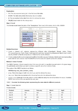
Step 3: Result
The formula would return the price of the “Smartphone” from row 2 of the table, which is Rs.100000/-

Related Exercises:
1 Create a dataset with columns representing different cities (Chandigarh, Bhopal, Indore, Patna,
Thiruvananthapuram, Kochi, Surat, Visakhapatnam) and rows representing temperature data for each month.
Use HLOOKUP to find the temperature in Patna for the month of March.
2 Create a dataset with columns representing different months (January, February, March) and rows representing
sales data for each product. Use HLOOKUP to find the sales of a specific product in January.

Method 3: Index Formula
The INDEX function in Excel is used to return the value of a cell in a specified row and column of a given range.
It is particularly useful when you want to retrieve a specific value from a table of data.
The syntax of the INDEX function is as follows:
INDEX(array, row_num, [column_num])
• array: This is the range of cells from which you want to retrieve the value.
• row_num: This is the row number within the array from which to retrieve the value.

• column_num: (Optional) This is the column number within the array from which to retrieve the value. If omitted,
INDEX returns the entire row specified by row_num.

TASK 1: Consider the following table representing the sales data for different products

Step 1: Create Data Set
Product Details

Product January February March April
Item A 100 120 80 150
Item B 75 90 110 85
Item C 120 100 130 95

Item D 90 80 75 110

436

CITS : IT & ITES - Computer Software Application - Exercise 72