Page 283 - CITS - Computer Software Application -TT

COMPUTER SOFTWARE APPLICATION - CITS

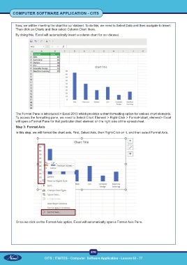
Now, we will be inserting the chart for our dataset. To do this, we need to Select Data and then navigate to Insert.
Then click on Charts and then select Column Chart there.
By doing this, Excel will automatically insert a column chart for our dataset.

The Format Pane is introduced in Excel 2013 which provides a chart formatting option for various chart elements.
To access the formatting pane, we need to Select Chart Element > Right-Click > Format<chart_element> Excel
will open a Format Pane for that particular chart element on the right side of the spreadsheet.

Step 3: Format Axis
In this step, we will format the chart axis. First, Select Axis, then Right-Click on it, and then select Format Axis.

Once we click on the Format Axis option, Excel will automatically open a Format Axis Pane.

270

CITS : IT&ITES - Computer Software Application - Lesson 63 - 77